Advance Filters

The best way to set up a sheet to use Advanced filters is to add a few rows above your data.

We will start with this data: Its the Invoice table from the famous Northwind Trading Company. (A Sample database provided by Microsoft)

And add a few rows at the top.

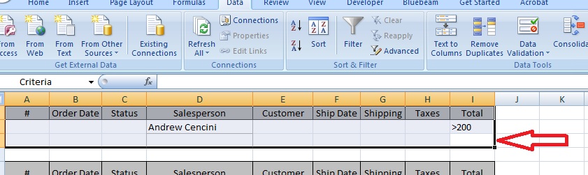
For this example we can add references in row 1 to mirror the tables headers in A4

Now we can add some criteria: For the names I like to just copy and paste data from the tables.

Copy both Andrew and Robert under the Salesperon header of the filter. Under Total I only want ones that are by Andrew AND greater than 100 OR by Robert AND greater than 200.

After adding the criteria we can apply the filter.

In the data tab, click advanced

The Advance filter window will pop up.

The list range, is the data in the table A5:I53

The criteria range is A1:I3 this will include the filter header and all rows below it that contain data.



Note: Be sure all of the rows you select in the filter data range contain data, or excel will include all results with no constraints. (It returns all of your data)

Click OK and now only the data were looking for is shown.



When you are finished reviewing the data or want to try another combination, press the clear button and try again.

Top Tip: When adding criteria 2 constraints in the same row will be calculated as AND, constraints in seperate rows will be calculated as OR. For our example above we are looking for invoices that were completed by Andrew AND were greater than 100, OR, by Robert AND greater than 200.





Calculating Filtered Values - The Subtotal

Excel filters are great, but wouldnt it be powerful to be able the to run calculations on the data as the filters change? The underutilized SUBTOTAL function should be added to your tool belt.

Syntax:
SUBTOTAL(Function,ref1,ref2,..)
There are seperate functions that will include or ignore Hidden values.
Note: Subtotal will automatically ignore any hidden data that is hidden becuase of the use of a filter.

Include Hidden Values	Function	Ignores Hidden Values
1	AVERAGE	101
2	COUNT	102
3	COUNTA	103
4	MAX	104
5	MIN	105
6	PRODUCT	106
7	STDEV	107
8	STDEVP	108
9	SUM	109
10	VAR	110
11	VARP	111

Lets look at an example:
The example below is counting the number of entries currently shown.

We have a list of fruit that we want to count.
In cell B2 the forumula =SUBTOTAL(103,C3:C35) will (CountA, the Range C3:C35), there are 33 records.

Note: CountA returns the number of non blank cells (Used to count cells with text or numbers)
          Count returns the number of cells that contain a number. (Used to count cells with numbers only)

If we add a filter to only show Apples and Oranges, this list shrinks.

The Subtotal is now 21, the calculation is ignoring the hidden data.

The next time your working with Filteres or hidden data, dont forget to make use of SUBTOTAL.

Counting Cell Background Colors

I have had several requests over the years for a function to count cells based on their background color.
Here is my solution. 2 Custom Functions.

If you dont know how to add a new function I will cover this in a later blog but for today we will skip that part.

The first function is CellColor and will help you identify the color index of a cell.

Function CellColor(CRange As Range)
 Dim cell As Range
        For Each cell In CRange
         CellColor = cell.Interior.ColorIndex
        Next cell
End Function

In the image above Cell B2 has the formula =Cellcolor(A2) which returns 38. Now we know what were looking for.

Now that we know the color of a cell we can use the next function CountColor to count the cells.

Function CountColor(CRange As Range, Color As Integer)
 Dim Ccount As Integer
 Dim cell As Range
        For Each cell In CRange
         If cell.Interior.ColorIndex = Color Then
         Ccount = Ccount + 1
         End If
        Next cell
        CountColor = Ccount  
End Function

 In the image above Cell B23 has the forumula =countcolor($A$2:$A$22,38) which returns 10.

Top Tip: Use them together and you don't have to remember that 38 is the index color of red.
=countcolor(A2:A22,CELLcolor(A2)) will return 10 as well.

First Post

Thanks for checking out my Excel blog. My goal here is to share the exciting world of Excel to everyone I can. If your looking for a solution to a problem send me a message and Ill be more than happy to help you out.